Convert a healthcare data range into a formatted Excel table with structured references, enabling automatic expansion and consistent formatting as new records are added (CO-6, CO-7)
Apply advanced sorting and multi-level filtering to a patient dataset to isolate specific record subsets needed for clinical reporting (CO-7)
Use VLOOKUP or XLOOKUP to retrieve patient information from a structured reference table, demonstrating correct syntax and error-handling for unmatched records (CO-6)
Evaluate which data summarization method (subtotals, PivotTable, or formula-based summary) best fits a given healthcare reporting need, explaining the trade-offs of each approach (CO-7)
Part 1 of 6
Part 1: Converting Data Ranges to Excel Tables
In the previous lesson, you learned that dedicated database systems manage large-scale healthcare data. Now let's use Excel as a lightweight database — with tables, lookups, and PivotTables that bring real analytical power to your desktop.
What Is an Excel Table?
An Excel Table is a structured data object that gives a range of cells special formatting, sorting, filtering, and formula capabilities. While a regular range of cells looks like a grid with data, an Excel Table adds intelligent structure: automatic headers, filter drop-downs on every column, consistent formatting, automatic expansion when you add new data, and a feature called structured references that makes formulas easier to read and maintain.
To convert a data range to an Excel Table:
Organize your data with column headers in the first row and one record per row below. Ensure there are no blank rows or columns within your data.
Select any cell within the data range.
Navigate to the Insert tab on the Ribbon and select Table, or use the keyboard shortcut Ctrl+T.
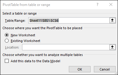
Excel detects the data range automatically. Verify the range in the dialog box and confirm that "My table has headers" is checked.
Select OK. Your data is now an Excel Table.
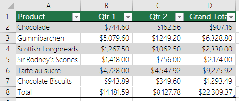
You will immediately notice several changes: the headers now display filter drop-down arrows, the rows display alternating color banding for readability, and a new Table Design tab appears on the Ribbon.
An Excel Table — notice the formatted headers, banded rows, and filter dropdown arrows — Microsoft Support
Excel Tables provide powerful features that plain ranges do not:
Automatic expansion — When you type data in the row immediately below the table or the column immediately to the right, Excel automatically extends the table to include the new data.
Table Styles — Dozens of pre-built styles accessible from the Table Design tab. Choose a style with navy headers and alternating white/light blue rows for professional healthcare reports.
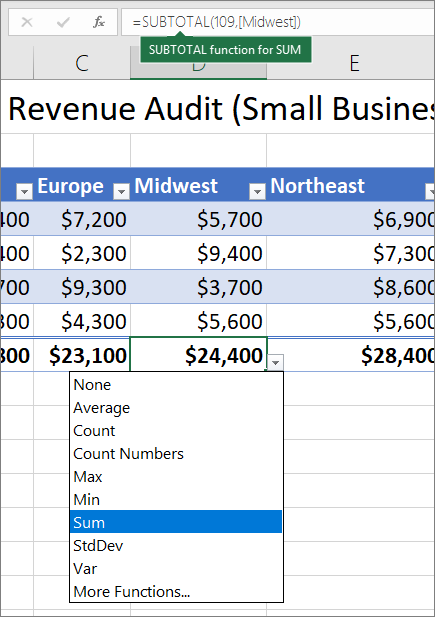
Totals Row — A built-in summary row at the bottom offering SUM, AVERAGE, COUNT, MIN, MAX, and other aggregate functions from a drop-down list.
The Total Row dropdown — choose from SUM, AVERAGE, COUNT, and other summary functions — Microsoft Support
Filter arrows — Every column header includes a drop-down for sorting and filtering without additional setup.
Inside an Excel Table, formulas use structured references instead of traditional cell addresses. Instead of writing =SUM(D2:D500), you write:
=SUM(PatientVisits[Charges])
Where PatientVisits is the table name and [Charges] is the column name. Structured references are self-documenting — anyone reading the formula can instantly understand what data it references. They also adjust automatically when the table expands or contracts, eliminating the common error of formulas missing newly added rows.
A calculated column uses the @ symbol to reference the current row: =TODAY()-[@LastVisitDate] calculates days since each patient's last visit across every row automatically.
Key Excel Table Features at a Glance
⊕
Auto-Expand
New rows and columns are automatically included in the table with all formatting and formulas applied.
[ ]
Structured Refs
Use column names in formulas instead of cell addresses for self-documenting, error-resistant formulas.
Σ
Totals Row
Built-in summary row with SUM, AVERAGE, COUNT, MIN, MAX from a simple drop-down.
▼
Filter Arrows
Every column gets sort and filter drop-downs automatically — no setup required.
▣
Table Styles
Dozens of professional formatting presets with alternating row colors, header styles, and borders.
Healthcare Connection
Healthcare Connection: A medical office manager maintains an Excel Table called SupplyOrders that tracks every medical supply purchase. Each time a new order arrives, she types the details in the next blank row, and the table automatically expands to include it. The Totals Row at the bottom shows the running total of all supply expenditures year-to-date. When the CFO asks for a spending report, the data is always current and complete without any manual formula adjustments.
Pro Tip
Pro Tip: Name your tables descriptively using the Table Design tab (e.g., PatientVisits, SupplyOrders, StaffSchedule). This makes structured references intuitive and formulas self-documenting across your workbook.
Part 2: Advanced Sorting and Filtering for Healthcare Data
Sorting and filtering are the most fundamental tools for exploring and analyzing data in an Excel Table. While basic single-column sorting is straightforward, healthcare data frequently requires multi-level sorting and advanced filtering to extract the specific records you need from large datasets.
Multi-level sorting arranges your data by multiple criteria in a priority sequence:
Select any cell in your Excel Table.
Navigate to the Data tab and select Sort.
Set your primary sort column, sort order, then select Add Level for secondary and tertiary criteria.
Example: Sort a patient visit log first by Department (alphabetical), then within each department by Visit Date (newest first), then by Patient Last Name (alphabetical). This three-level sort organizes thousands of records into a structured, easy-to-navigate format.
Excel supports custom sort orders for when alphabetical or numerical ordering is not appropriate. For example, sorting urgency levels as "Critical, High, Medium, Low" instead of alphabetically (which would place "Low" before "Medium"). Create a custom list in Excel's options and reference it in the Sort dialog.
Every column in an Excel Table automatically includes AutoFilter drop-down arrows. Select the arrow on any column header to see all unique values. Check or uncheck values to show only matching records.
Example: Select the Department filter and choose only "Cardiology" to instantly hide all rows except Cardiology visits.
For complex filtering needs, access Number Filters, Text Filters, or Date Filters through the AutoFilter arrow:
Equals / Does Not Equal – Match or exclude specific values.
Greater Than / Less Than – Filter by threshold (e.g., charges greater than $500).
Between – Filter date or value ranges (e.g., visits between Jan 1 and Mar 31).
Contains / Begins With / Ends With – Partial text matches (e.g., diagnoses containing "diabetes").
Top 10 / Above Average – Filter for highest values or values above the column average.
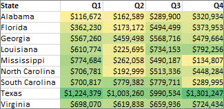
If you have applied conditional formatting to your table (such as highlighting overdue follow-ups in red or flagging abnormal lab values with icons), you can filter by cell color or icon. This is powerful for quickly isolating records that need attention — for example, showing only patients with red-flagged overdue appointments.
Color scales provide instant visual analysis — darker colors indicate higher values, making patterns easy to spot — Microsoft Support
Filters across multiple columns work together with AND logic: a record must meet all active filter criteria to appear. If you filter Department to "Pediatrics" AND Visit Date to the current month AND Insurance to "Medicaid," only records matching all three conditions will display.
This multi-column filtering capability makes Excel Tables a practical tool for ad hoc healthcare data analysis.
Healthcare Connection
A billing coordinator needs to review all denied insurance claims for the Orthopedics department submitted in the past 90 days. By applying three filters — Department equals "Orthopedics," Claim Status equals "Denied," and Submission Date is within the last 90 days — the coordinator instantly isolates the relevant records from thousands of claims for efficient review and resubmission.
Try It Yourself
Try It Yourself: Open an Excel Table with patient data. Apply a multi-level sort by Department, then Visit Date. Next, use AutoFilter to show only a single department and add a date filter for the current month. Notice how quickly you can isolate exactly the records you need.
Part 3 of 6
Part 3: VLOOKUP and XLOOKUP: Retrieving Healthcare Data
One of the most common tasks in healthcare data management is looking up information from one table based on a value you already know. For example, given a Patient ID, you need to pull the patient's name, insurance plan, or primary physician from a master patient list. The VLOOKUP and XLOOKUP functions are Excel's primary tools for this type of data retrieval.
VLOOKUP (Vertical Lookup) searches for a value in the first column of a range and returns a value from a specified column in the same row:
lookup_value – The value to search for (e.g., a Patient ID).
table_array – The range or table containing the data.
col_index_num – The column number containing the return value (1 = lookup column).
range_lookup – Use FALSE for exact match (almost always correct for healthcare data).
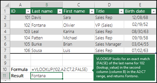
Example:=VLOOKUP(A2, PatientMaster, 5, FALSE) — looks up the Patient ID in A2 and returns column 5 (Insurance).
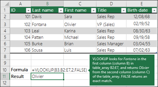
VLOOKUP searches the first column of a range and returns a value from another column — here it finds "Fontana" and returns "Olivier" — Microsoft Support
XLOOKUP, introduced in Microsoft 365, addresses all of VLOOKUP's limitations and is the recommended function for new work:
return_array – The single column containing the return values.
if_not_found – A custom message instead of #N/A error.
match_mode – 0 for exact match (default).
search_mode – 1 for first-to-last (default), -1 for last-to-first.
Example:=XLOOKUP(A2, PatientMaster[Patient_ID], PatientMaster[Insurance], "Patient Not Found")
Key differences at a glance:
Direction: VLOOKUP searches only the first column; XLOOKUP searches any column and returns from any other column.
Error handling: VLOOKUP returns #N/A (requires IFERROR wrapper); XLOOKUP has a built-in if_not_found parameter.
Default match: VLOOKUP defaults to approximate match (risky!); XLOOKUP defaults to exact match (safer).
Column reference: VLOOKUP uses a fragile numeric index; XLOOKUP uses named column references.
Availability: VLOOKUP works in all Excel versions; XLOOKUP requires Microsoft 365 or Excel 2021+.
Recommendation: Use XLOOKUP for all new healthcare data work in Microsoft 365. Use VLOOKUP only when working with older Excel versions.
Searches only the first column – The lookup value must be in the leftmost column of the table_array.
Returns only to the right – Cannot look left of the lookup column.
Column index is a number – A hard-coded number makes formulas fragile if columns are inserted or deleted.
Returns only the first match – If there are duplicate lookup values, VLOOKUP returns only the first occurrence.
Always use exact match (FALSE in VLOOKUP, 0 in XLOOKUP) when looking up patient IDs or MRNs. Approximate matching can return incorrect patient data — a serious safety risk.
Handle errors gracefully – Use XLOOKUP's if_not_found parameter or wrap VLOOKUP in IFERROR to display meaningful messages instead of #N/A.
Verify results – After building lookup formulas, spot-check several results against the source table to confirm accuracy before using the data for reports or decisions.
VLOOKUP vs. XLOOKUP Comparison
Feature
VLOOKUP
XLOOKUP
Lookup Direction
First column only; returns right
Any column; returns from any column
Column Reference
Numeric index (fragile)
Column name references (robust)
Error Handling
#N/A; requires IFERROR wrapper
Built-in if_not_found parameter
Default Match
Approximate (TRUE)
Exact (0)
Multiple Returns
One value per formula
Can return entire row or multiple columns
Search Direction
Top-to-bottom only
First-to-last, last-to-first, binary
Availability
All Excel versions
Microsoft 365 and Excel 2021+
Recommendation
Legacy or older Excel versions
Preferred for all new work
=VLOOKUP(102, A2:C7, 2, FALSE) — looks up ID 102 and returns the corresponding name from column 2 — Microsoft Support
Healthcare Connection
A front-desk coordinator is preparing 200 appointment reminder letters. She has Patient IDs but needs each patient's full name and phone number. Using XLOOKUP, she pulls First_Name, Last_Name, and Phone from the master patient table in seconds. The "Patient Not Found" fallback immediately highlights three records with invalid Patient IDs, which she flags for correction before the letters go out — preventing reminder calls to the wrong patients.
When working with large healthcare datasets, you often need to see summary statistics for groups within your data — total charges by department, average wait time by provider, or patient count by insurance type. Excel's Subtotal feature automates this process by inserting summary rows at each group boundary in your sorted data.
Subtotals require your data be sorted by the grouping column first. To apply:
Sort your data by the column you want to group by (e.g., Department).
Select any cell in the data range.
Navigate to the Data tab and select Subtotal.
In the Subtotal dialog box, set:
At each change in: Select the grouping column (Department).
Use function: Choose SUM, COUNT, AVERAGE, etc.
Add subtotal to: Check the columns to subtotal (e.g., Charges, Visit Count).
Select OK. Excel inserts subtotal rows and adds outline levels.
Note: Subtotals work on regular ranges, not Excel Tables. You may need to convert your table back to a range first.
The Subtotal button on the Data tab — automatically groups and summarizes data — Microsoft Support
After applying subtotals, Excel displays outline level buttons (1, 2, 3) in the left margin:
Level 1 – Shows only the grand total.
Level 2 – Shows group subtotals and the grand total (the summary view).
Level 3 – Shows all individual records plus subtotals (the detail view).
Level 2 is especially useful for management reports — a concise summary of charges or visit counts by department without scrolling through hundreds of records.
Outline level buttons (1, 2, 3) let you expand or collapse subtotal groups — Microsoft Support
The SUBTOTAL function can ignore hidden rows (rows hidden by filtering), making it ideal for summarizing filtered data:
=SUBTOTAL(function_num, ref1, [ref2], ...)
Common function numbers: 1 (AVERAGE), 2 (COUNT), 3 (COUNTA), 4 (MAX), 5 (MIN), 9 (SUM). Using 109 instead of 9 calculates a SUM that excludes manually hidden rows.
Example: After filtering to show only Cardiology visits, =SUBTOTAL(109, E:E) calculates the sum of charges for only the visible Cardiology rows.
Healthcare Connection
Healthcare Connection: A department manager needs to present a summary of patient visit charges by department for the quarterly budget meeting. After sorting by Department and applying subtotals on the Charges column, she selects Outline Level 2 to see: Emergency $245,000, Cardiology $189,000, Orthopedics $156,000, Primary Care $312,000, Pediatrics $98,000, with a Grand Total of $1,000,000. This one-page summary, generated in seconds, provides exactly the detail the budget committee needs.
Analysis Tool Selector
Pick the right Excel tool for each healthcare data challenge — 6 real-world scenarios
Patient Visit Log5,000 rows
Patient ID
Last Name
Dept
Insurance
Charges
P-1001
Garcia
Cardiology
Medicare
$425
P-1002
Johnson
Ortho
BlueCross
$850
P-1003
Williams
Primary
Medicare
$175
... 4,997 more rows
Task 1 of 6
★ 0/0
Find all patients with "Medicare" insurance in a 5,000-row visit log.
Which Excel tool is the best choice?
0/6
Tools Selected Correctly
Part 5 of 6
Part 5: PivotTables: Powerful Healthcare Data Summaries
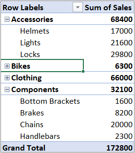
If Subtotals provide a straightforward grouped summary, PivotTables take data summarization to an entirely different level. A PivotTable is an interactive data analysis tool that lets you reorganize, summarize, filter, and analyze large datasets by dragging fields into different areas. PivotTables are arguably the single most powerful feature in Excel for healthcare data analysis.
PivotTables transform detailed records into summary views — drag fields to Rows, Columns, Values, and Filters — Microsoft Support
Healthcare Connection: At the end of each quarter, the clinic's operations analyst creates a PivotTable summarizing 25,000 patient visits. The director first asks to see total visits by department and month. Then: "Show me only Medicare patients." The analyst drags Insurance_Type to the Filters area and selects Medicare. Next: "Now show average charges instead of total." A right-click, change Sum to Average, and the entire report recalculates. Three different analytical views of 25,000 records, generated in under a minute.
Pro Tip
You can drag the same field to the Values area twice — once set to SUM and once set to COUNT — to see both total charges and visit counts side by side in the same PivotTable.
PivotCharts provide a visual representation of PivotTable data — changes to one are reflected in the other — Microsoft Support
Part 6 of 6
Part 6: Excel Database Best Practices for Healthcare
Throughout this lesson, you have learned to use Excel Tables, advanced sorting and filtering, lookup functions, subtotals, and PivotTables — a powerful toolkit for managing and analyzing healthcare data. To use these tools effectively and safely, keep the following best practices in mind.
Data Organization Principles
☐
One Record Per Row
No merged cells, no blank rows for spacing, no multiple data points in a single cell.
Aa
Consistent Entry
Same spelling, abbreviation, and formatting. "Cardiology" vs "Cardio" vs "CARDIOLOGY" = 3 departments in a PivotTable.
☑
Data Validation
Use drop-down lists for Department, Insurance_Type, Visit_Type to prevent misspellings at the source.
#
Unique Identifier
Every table needs a unique ID column (Patient ID, Appointment ID, Claim Number) to enable lookups.
🔒
PHI Security
Encrypt files with PHI, use SharePoint with permissions, never email unencrypted patient data.
Be mindful of PHI – If your Excel file contains Protected Health Information, store files on encrypted, access-controlled drives. Never email unencrypted PHI. Use Excel's password protection and file encryption features.
Limit access – Share through SharePoint or OneDrive with appropriate permissions rather than emailing copies.
Do not use Excel as a permanent clinical database – Excel is excellent for departmental tracking and ad hoc analysis. It is not a substitute for a HIPAA-compliant EHR or practice management system.
Export PivotTable results by copying and pasting as values into a new worksheet, then sharing without the source data.
Save as PDF for reports that recipients should not modify.
Remove sensitive columns before sharing. Strip patient names or IDs and include only de-identified aggregate data.
A calculated column is a column in an Excel Table where every cell contains the same formula, automatically applied to every row. Type a formula in one cell of an empty table column, and Excel fills the entire column.
Example:=TODAY()-[@LastVisitDate] — The @ symbol means "the value in this row." This calculates days since last visit for every patient automatically.
Key Takeaway
Excel Tables, lookup functions, subtotals, and PivotTables transform Excel from a simple spreadsheet into a genuine data analysis platform. Combined with proper data organization, validation, and PHI security practices, these tools enable healthcare professionals to generate insights from operational data quickly and accurately — without needing a dedicated database system for every analysis task.
Healthcare Connection
A clinic compliance officer exports de-identified patient visit data from the EHR into an Excel Table for a quality audit. She uses XLOOKUP to match diagnosis codes to quality measure criteria, creates a PivotTable to summarize compliance rates by provider and quarter, and exports the PivotTable summary as a PDF for the audit committee. The original data file remains on the clinic's encrypted SharePoint site with restricted access. The shared PDF contains only aggregate statistics with no individual patient identifiers — maintaining HIPAA compliance while enabling data-driven quality improvement.
Knowledge Check
A healthcare office manager converts a patient visit data range to an Excel Table. She types a new record in the row immediately below the last table row. What happens automatically?
Correct! One of the key advantages of Excel Tables is automatic expansion. When you type data in the row immediately below the last table row, Excel automatically extends the table to include the new data. All table formatting, filter settings, structured references, and calculated column formulas are automatically applied to the new row.
Not quite. The correct answer is that the table automatically expands to include the new row with all formatting and formulas applied. This is one of the most valuable features of Excel Tables — no manual adjustments needed when your dataset grows.
Knowledge Check
A medical assistant has a list of Patient IDs and needs to retrieve each patient's primary physician from a master patient table called PatientDirectory. Which XLOOKUP formula correctly retrieves the physician name for the Patient ID in cell A2?
Correct! The XLOOKUP formula is =XLOOKUP(A2, PatientDirectory[Patient_ID], PatientDirectory[Primary_MD], "Not Found"). The first argument (A2) is the lookup value, the second specifies where to search (Patient_ID column), the third specifies where to return from (Primary_MD column), and the fourth provides a friendly message if no match is found.
Not quite. The correct formula is =XLOOKUP(A2, PatientDirectory[Patient_ID], PatientDirectory[Primary_MD], "Not Found"). Option A reverses the lookup and return arrays. Option C uses VLOOKUP incorrectly with a column name in quotes. Option D places the lookup_array as the first argument.
Knowledge Check
A clinic analyst is building a PivotTable from 15,000 patient visit records. The clinic director wants to see total charges broken down by department (rows) and month (columns), with the ability to filter the entire report by insurance type. Where should the analyst place the Insurance_Type field?
Correct! The Filters area creates a report-level drop-down filter at the top of the PivotTable. Placing Insurance_Type there allows the director to select a specific insurance type and have the entire PivotTable recalculate, while maintaining the Department (rows) by Month (columns) layout.
Not quite. The correct answer is the Filters area. It creates a report-level drop-down that filters the entire PivotTable. Placing it in Rows would add sub-rows, in Columns would add sub-columns, and in Values would count it rather than filter by it.
Lesson 5.3 Summary
Excel Tables add structured references, automatic expansion, filter arrows, and a Totals Row to transform plain ranges into powerful data management tools.
Multi-level sorting and advanced filtering (text, number, date, color) let you isolate specific healthcare records from large datasets.
VLOOKUP retrieves data from the first column of a range; XLOOKUP is the modern replacement with flexible lookup direction, built-in error handling, and named column references.
Subtotals with outline levels provide grouped summaries (by department, provider, etc.) with one-click detail expansion.
PivotTables are Excel's most powerful analysis tool — drag fields into Rows, Columns, Values, and Filters to generate interactive multi-dimensional reports in seconds.
Proper data organization (one record per row, consistent entry, data validation, unique IDs) and PHI security practices are essential for reliable healthcare data management in Excel.