Construct formulas using arithmetic operators and cell references to calculate healthcare metrics such as total costs, average wait times, or staffing ratios (CO-6)
Given a formula that produces incorrect results when copied, diagnose the cell reference error and apply the correct absolute or relative reference to fix it (CO-6)
Apply SUM, AVERAGE, COUNT, MIN, MAX, and IF functions to summarize a healthcare dataset and flag records that meet specified clinical criteria (CO-6)
Sort and filter a patient or inventory dataset by multiple criteria to isolate specific subsets needed for reporting or decision-making (CO-7)
Part 1 of 6
Part 1 of 6 — Formula Basics: Operators and Order of Operations
The true power of Excel lies not in storing data, but in calculating with it. A formula is an instruction that tells Excel to perform a calculation using values, cell references, and operators. Every formula in Excel begins with an equals sign (=). When Excel sees the equals sign, it knows that what follows is a calculation to evaluate, not just text or a number to display.
Arithmetic Operators
Excel uses standard arithmetic operators to perform calculations:
+ (Addition) – Adds values. Example: =B2+C2 adds the values in cells B2 and C2.
- (Subtraction) – Subtracts one value from another. Example: =D2-E2 calculates the difference.
* (Multiplication) – Multiplies values. Example: =F2*G2 multiplies the values in cells F2 and G2.
/ (Division) – Divides one value by another. Example: =H2/I2 divides the value in H2 by I2.
^ (Exponentiation) – Raises a number to a power. Example: =J2^2 squares the value in J2.
Order of Operations (PEMDAS)
When a formula contains multiple operators, Excel follows the mathematical order of operations, remembered by the acronym PEMDAS:
Parentheses – Operations inside parentheses are calculated first.
Exponents – Powers and roots are calculated next.
Multiplication and Division – Calculated left to right.
Addition and Subtraction – Calculated left to right.
This matters in healthcare calculations. Consider a formula to calculate a patient's Body Mass Index (BMI): BMI = weight (kg) / height (m) squared. In Excel, if weight is in cell B2 and height in meters is in cell C2, the formula would be =B2/C2^2. Excel first calculates C2^2 (height squared), then divides B2 by that result. To be explicit, you can use parentheses: =B2/(C2^2).
Building Your First Formula
The formula bar displays the contents of the active cell — type formulas directly here or in the cell itself — Microsoft Support
To enter a formula:
Select the cell where you want the result to appear.
Type the equals sign (=).
Type the formula using cell references and operators (e.g., =B2+C2).
Press Enter to confirm. Excel displays the calculated result in the cell.
Instead of typing cell references, you can select cells while building a formula. After typing the equals sign, select cell B2 (Excel inserts B2 into the formula), type the operator (+), then select cell C2. This point-and-select method reduces errors, especially in large worksheets.
Every Excel formula can contain four elements: functions, cell references, constants, and operators — Microsoft Support
Functions — predefined formulas like PI() that return calculated values
References — cell addresses like A2 that pull values from other cells
Constants — numbers or text typed directly into the formula
Operators — symbols like + (add), * (multiply), and ^ (power)
Excel also supports comparison operators that return TRUE or FALSE:
= (Equal to) – =A2=B2 returns TRUE if the values match.
<> (Not equal to) – Returns TRUE if values differ.
> (Greater than) and < (Less than)
>= (Greater than or equal to) and <= (Less than or equal to)
These operators are critical for the IF function you will learn later in this lesson, where you need Excel to make decisions based on whether values meet certain criteria — such as whether a blood pressure reading exceeds a clinical threshold.
Healthcare Connection
A pharmacy technician needs to calculate the total cost of a prescription: the per-unit price in cell B2 multiplied by the quantity in cell C2, minus the insurance discount in cell D2. The formula =B2*C2-D2 follows the correct order of operations: multiplication first (B2*C2), then subtraction of the discount (D2). Using parentheses for clarity — =(B2*C2)-D2 — makes the formula easier for a colleague to understand.
Part 2 of 6
Part 2 of 6 — Relative, Absolute, and Mixed Cell References
Understanding how Excel handles cell references when you copy formulas is one of the most important concepts in spreadsheet design. According to Microsoft's documentation, there are three types of cell references: relative, absolute, and mixed. Each behaves differently when a formula is copied from one cell to another.
Relative References (Default) – A reference like A1 tells Excel to look at a cell in a relative position from the formula cell. When you copy a formula containing a relative reference, the reference automatically adjusts based on the new location.
Cell C2 contains the formula =A2+B2.
When copied to C3, Excel adjusts it to =A3+B3.
When copied to C4, it becomes =A4+B4.
This is exactly what you want in most situations. If column A contains patient systolic blood pressure and column B contains diastolic, a formula in column C that calculates the difference (=A2-B2) should adjust for each row as you copy it down.
Relative references automatically adjust when you copy a formula — the reference shifts relative to its new position — Microsoft Support
Absolute References – Use dollar signs to lock a cell address so it does not change when the formula is copied. The syntax is $A$1. The dollar sign before the column letter locks the column; the dollar sign before the row number locks the row.
Cell F1 contains a tax rate of 8.5% that applies to all items.
Cell F2 contains the formula =E2*$F$1.
When copied to F3, F4, F5, etc., E2 adjusts (E3, E4, E5) but $F$1 stays locked on cell F1.
Without the dollar signs, copying the formula would change F1 to F2, F3, and so on — pointing to empty cells and producing errors.
Absolute references (with $ signs) lock a cell address so it doesn't change when copied — essential for lookup tables and fixed rates — Microsoft Support
Mixed References – Lock either the row or the column, but not both:
$A1 – The column (A) is locked; the row adjusts when copied.
A$1 – The row (1) is locked; the column adjusts when copied.
Mixed references are used in more advanced formulas, such as lookup tables or matrices where you need one dimension to stay fixed while the other changes.
The F4 Shortcut – While editing a formula, place the cursor on a cell reference and press F4 to cycle through reference types:
First press: $A$1 (absolute)
Second press: A$1 (mixed — row locked)
Third press: $A1 (mixed — column locked)
Fourth press: A1 (relative, back to default)
This shortcut is far faster than manually typing dollar signs and is essential for building accurate formulas efficiently.
Healthcare Connection
Healthcare Connection: A medical office manager is calculating the total cost of supplies for multiple departments. Column E lists the item cost before tax, and cell G1 contains the sales tax rate (7.5%). The formula in F2 is =E2*$G$1. Using an absolute reference for the tax rate cell ensures that when the formula is copied down for all 50 items, every row correctly multiplies its item cost by the same tax rate in G1. If the tax rate changes, updating cell G1 once automatically recalculates all 50 rows.
▶
Excel Formulas Full Course• 120 min
Part 3 of 6
Part 3 of 6 — Essential Excel Functions: SUM, AVERAGE, COUNT, MIN, MAX
While formulas using arithmetic operators are powerful, Excel's built-in functions simplify common calculations dramatically. A function is a predefined formula that performs a specific calculation. Every function follows the same basic syntax:
=FUNCTIONNAME(argument1, argument2, ...)
The arguments inside the parentheses tell the function which cells or values to use. Let's examine the five most essential functions for healthcare data analysis.
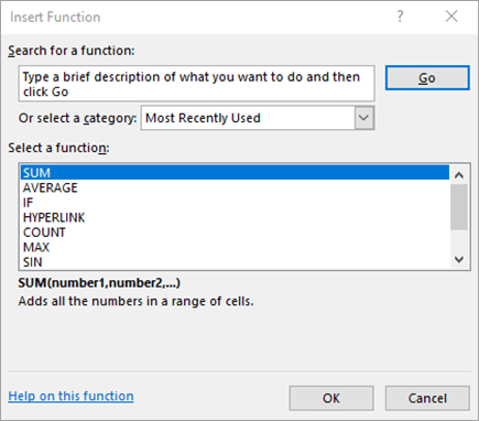
Select a cell range when entering a function — Excel highlights the referenced cells in color — Microsoft SupportThe Insert Function dialog (Shift+F3) — search for functions or browse by category — Microsoft Support
The SUM function adds all numbers in a specified range:
=SUM(number1, [number2], ...)
The most common usage is to sum a continuous range: =SUM(B2:B50) adds all values from B2 through B50. You can also sum multiple ranges: =SUM(B2:B50, D2:D50).
Healthcare example: Calculate the total number of patient visits across all weekdays. If cells B2 through B6 contain the daily visit counts for Monday through Friday, =SUM(B2:B6) returns the weekly total.
The AVERAGE function calculates the arithmetic mean of a range of numbers:
=AVERAGE(number1, [number2], ...)
Healthcare example: Calculate the average patient wait time. If column C contains wait times in minutes for 30 patients, =AVERAGE(C2:C31) returns the average wait time. This metric is commonly tracked to monitor operational efficiency and patient satisfaction.
COUNTA counts all non-empty cells, regardless of content: =COUNTA(value1, [value2], ...)
Healthcare example: Count how many patients have recorded blood pressure readings this month. If column D contains systolic BP readings but some cells are blank, =COUNT(D2:D100) returns only cells with numeric entries. Use =COUNTA(A2:A100) to count patient name entries (text values) in the roster.
MIN returns the smallest value, and MAX returns the largest:
Healthcare example: Identify the shortest and longest patient wait times. If column C contains wait times, =MIN(C2:C31) returns the shortest wait and =MAX(C2:C31) returns the longest. Clinic managers use these alongside the average to understand the full range of the patient experience.
AutoSum is a toolbar shortcut that inserts the SUM function automatically. Select a cell directly below or to the right of a column or row of numbers, then select the AutoSum button (the Greek sigma symbol Σ on the Home tab). Excel guesses the range and inserts =SUM(...).
You can also use the keyboard shortcut Alt+= (press Alt and the equals sign simultaneously) to trigger AutoSum. Select the AutoSum drop-down arrow to choose AVERAGE, COUNT, MIN, or MAX instead.
Function
Syntax
What It Does
Healthcare Example
SUM
=SUM(range)
Adds all numbers in the specified range
=SUM(B2:B31) totals monthly patient visits across 30 days
AVERAGE
=AVERAGE(range)
Calculates the arithmetic mean of a range
=AVERAGE(C2:C31) finds the average patient wait time in minutes
COUNT
=COUNT(range)
Counts cells containing numeric values
=COUNT(D2:D100) counts patients with recorded BP readings
COUNTA
=COUNTA(range)
Counts all non-empty cells (numbers and text)
=COUNTA(A2:A100) counts patient name entries in the roster
MIN
=MIN(range)
Returns the smallest value in a range
=MIN(C2:C31) identifies the shortest patient wait time
MAX
=MAX(range)
Returns the largest value in a range
=MAX(C2:C31) identifies the longest patient wait time
IF
=IF(test, true, false)
Returns one value if TRUE, another if FALSE
=IF(D2>140,"HIGH","Normal") flags elevated systolic BP
AutoSum
Alt+= or Σ button
Shortcut that auto-inserts SUM (or others)
Select below copay amounts, press Alt+= to total instantly
Healthcare Connection
Healthcare Connection: A clinic's front desk manager tracks daily patient wait times in an Excel spreadsheet. At the end of the month, they use =AVERAGE(C2:C31) to report the average wait time (target: under 15 minutes), =MAX(C2:C31) to identify the worst wait (for process improvement), =COUNT(C2:C31) to confirm the number of data points, and =SUM(B2:B31) to total all patient visits. These four functions transform raw data into actionable metrics for clinic leadership.
Part 4 of 6
Part 4 of 6 — The IF Function: Conditional Logic for Healthcare Decisions
The IF function is one of the most powerful and widely used functions in Excel because it enables your spreadsheet to make decisions. According to Microsoft's official documentation, the IF function checks whether a condition is true or false, then returns one value if TRUE and a different value if FALSE.
IF Function Syntax
The syntax of the IF function is:
=IF(logical_test, value_if_true, value_if_false)
logical_test – The condition to evaluate. Typically a comparison using operators like >, <, =, >=, <=, or <>.
value_if_true – The value returned if the condition is TRUE.
value_if_false – The value returned if the condition is FALSE.
Step-by-Step: Building a Blood Pressure Alert
You have a patient vitals spreadsheet where column D contains systolic blood pressure readings. You want column E to display "HIGH" if the systolic BP is 140 or above and "Normal" if below 140.
Select cell E2 (next to the first patient's systolic reading in D2).
Type the equals sign: =
Type the function name: IF(
Enter the logical test: D2>=140 — checks whether systolic reading is 140 or higher.
Type a comma and enter the value if true: "HIGH" — text values must be enclosed in quotation marks.
Type another comma and enter the value if false: "Normal"
The value_if_true and value_if_false arguments can be numbers, cell references, or even other formulas:
=IF(C2>60, C2*0.10, 0) – If a patient's outstanding balance exceeds $60, calculate a 10% late fee; otherwise $0.
=IF(B2="Yes", 1, 0) – If a consent form column says "Yes," assign 1 (complete); otherwise 0. Summing this column gives a total count of completed forms.
You can place one IF function inside another to handle multiple conditions. This is called nesting. To categorize blood pressure readings into three levels:
This formula first checks if D2 is 140 or above (HIGH). If not, it checks if D2 is 120 or above (Elevated). If neither, it returns "Normal." You can nest up to 64 IF functions, but for readability, try to limit nesting to two or three levels.
Missing quotation marks around text – =IF(D2>=140,HIGH,Normal) without quotes will cause Excel to look for cell ranges named HIGH and Normal, likely returning an error.
Missing comma between arguments – Each of the three arguments must be separated by a comma.
#VALUE! error – Often caused by comparing a text cell to a number, or vice versa. Ensure the data types match the logical test.
Healthcare Connection
Healthcare Connection: The IF function is invaluable for clinical alert systems. A nurse reviewing patient vitals can use =IF(G2<95,"LOW O2 - ALERT","OK") in the SpO2 column to flag patients with oxygen saturation below 95%. Combined with conditional formatting (from Lesson 4-1), the IF function creates a simple but effective monitoring tool that draws immediate attention to patients who may need intervention.
Part 5 of 6
Part 5 of 6 — Sorting Data for Healthcare Insights
Once your spreadsheet contains data and formulas, you need tools to organize and explore that data. Sorting rearranges your data rows based on the values in one or more columns, making it easier to identify patterns, find specific records, and prepare data for reports.
Single-Column Sort
The simplest sort rearranges data based on one column:
Select any cell in the column you want to sort by.
Go to Home > Sort & Filter or Data > Sort.
Choose Sort A to Z (ascending) or Sort Z to A (descending).
For text, ascending means alphabetical order (A to Z); for numbers, ascending means smallest to largest; for dates, ascending means oldest to newest.
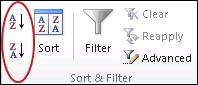
The Sort buttons on the Data tab let you quickly sort data in ascending (A→Z) or descending (Z→A) order — Microsoft Support
Multi-Column Sort
Multi-column sorting lets you sort by a primary column, then by a secondary column within ties. For example, sort patients first by department, then alphabetically by last name within each department.
Select any cell in your data range.
Go to Data > Sort to open the Sort dialog box.
Set the first sort level: Sort by Department, Order A to Z.
Select Add Level to add a second sort: Then by Last Name, Order A to Z.
Select OK.
Best Practice
Ensure your data has headers – Check the "My data has headers" box in the Sort dialog so Excel does not sort your header row into the data. Also avoid blank rows or columns — blanks can cause Excel to sort only a portion of your data, separating related records.
Healthcare Connection
Healthcare Connection: A clinic manager reviewing patient wait times sorts the data by wait time in descending order to identify the longest waits. Then, using a multi-column sort, they sort by appointment type (routine vs. urgent) and then by wait time within each type. This analysis reveals whether urgent patients are being prioritized appropriately or whether all patients experience similar delays.
Part 6 of 6
Part 6 of 6 — Filtering Data and Data Validation
While sorting rearranges all your data, filtering temporarily hides rows that do not meet specific criteria, letting you focus on a subset. Excel's AutoFilter feature is the primary tool for filtering data.
Using AutoFilter
To enable AutoFilter:
Select any cell within your data range.
Go to Data > Filter (or Home > Sort & Filter > Filter).
Drop-down arrows appear in each header cell.
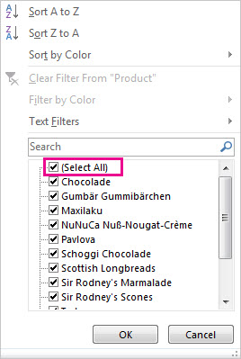
Click the filter arrow in a column header to select which values to show or hide — Microsoft Support
Checkboxes – Check or uncheck specific values. In a Department column, uncheck all except "Cardiology" to see only cardiology patients.
Text Filters – Filter text columns by "Contains," "Begins With," "Equals," etc. Example: Filter patient names that begin with "S" to quickly locate a record.
Number Filters – Filter numeric columns by "Greater Than," "Less Than," "Between," "Top 10," etc. Example: Filter systolic BP for readings greater than 140 to identify patients needing follow-up.
Custom Filters – Combine two conditions with AND or OR logic. Examples:
Systolic BP greater than 140 AND less than 180 (hypertension stage 2 range).
Department equals "Emergency" OR "Urgent Care."
A filtered column's drop-down arrow changes to a funnel icon, reminding you that a filter is active. To clear a filter, select the funnel icon and choose Clear Filter From [Column Name]. Filtering hides rows but does not delete them — all hidden data remains in the worksheet.
Data Validation Basics
Data validation restricts the type of data that can be entered into specific cells, reducing errors at the point of entry. This is particularly important in healthcare, where accurate data entry can impact patient care and billing.
Select the cells where you want to restrict entry.
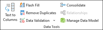
Go to Data > Data Validation.
Choose a validation type: Whole Number, Decimal, Date, Time, Text Length, or List.
Set the criteria (e.g., Whole Number between 50 and 250 for systolic BP readings).
Optionally, add an Input Message (a tooltip that guides the user) and an Error Alert (shown when invalid data is entered).
Access Data Validation from the Data tab to control what users can enter in cells — Microsoft Support
Named Ranges for Clarity
A named range assigns a descriptive name to a cell or range of cells, making formulas easier to read. Instead of =SUM(C2:C31), name the range C2:C31 as WaitTimes and write =SUM(WaitTimes). To create a named range: select the range, click in the Name Box (left of the formula bar), type a descriptive name, and press Enter.
Healthcare Connection
A medical records coordinator needs to find all patients seen in the Emergency department during January 2026 with systolic blood pressure above 140. Using AutoFilter, they filter the Department column for "Emergency," the Date column for January 2026, and the Systolic BP column for values greater than 140. Within seconds, the spreadsheet displays only matching records — a task that would take much longer scrolling through hundreds of rows manually. Data validation on the Department column ensures every entry is one of the approved department names, preventing filtering errors caused by inconsistent data entry like "ER" versus "Emergency."
Formula Builder: Healthcare Calculations
5 challenges — Select the correct formula for each healthcare scenario
X
Healthcare Data Workbook
C16
fx
Challenge
★ 0/0Challenge 1 of 5
Select the correct formula
Formula Builder Score
Knowledge Check
A medical office manager has a supply order spreadsheet with item costs in column C and a single sales tax rate in cell F1. The formula in D2 is =C2*F1. When copied to D3, it becomes =C3*F2, which produces an error because F2 is empty. What should the manager change in the original formula to prevent this error?
Correct! The tax rate in cell F1 is a constant value that should not change when the formula is copied down. Using an absolute reference ($F$1) locks the reference so it always points to the tax rate cell. The item cost reference (C2) should remain relative so it adjusts to C3, C4, etc. for each row's item cost.
Not quite. The correct answer is to change F1 to $F$1. The tax rate is a constant that should stay locked when the formula is copied. The item cost (C2) should remain relative so it adjusts for each row.
Knowledge Check
A clinic manager wants to determine how many patients out of 50 have recorded blood pressure readings this month. Some cells in the blood pressure column contain numbers, but cells for patients not yet seen are blank. Which function should the manager use?
Correct! COUNT specifically counts cells that contain numeric values, ignoring blank cells and text. Since the blood pressure column contains numbers for patients with readings and blank cells for patients not yet seen, COUNT returns the correct number of recorded readings.
Not quite. The correct function is COUNT, which specifically counts cells with numeric values. COUNTA would also count text entries, SUM adds values rather than counting, and AVERAGE calculates the mean.
Knowledge Check
A nurse needs an Excel formula that displays "FEVER" if a patient's temperature in cell G2 is 100.4 or higher, and "Normal" otherwise. Which formula is correct?
Correct! The correct IF syntax is =IF(logical_test, value_if_true, value_if_false). The logical test G2>=100.4 checks whether the temperature is 100.4 or higher. Text values like "FEVER" and "Normal" must be enclosed in quotation marks.
Not quite. The correct formula is =IF(G2>=100.4,"FEVER","Normal"). The IF syntax requires (logical_test, value_if_true, value_if_false) — text must be in quotation marks, and the arguments must be in the correct order.
Knowledge Check
A clinic manager has a spreadsheet with 500 patient visit records. She needs to find all patients in the Cardiology department who had a wait time over 30 minutes during January 2026. What is the MOST efficient approach?
Correct! AutoFilter is the most efficient tool because it allows you to apply multiple criteria simultaneously — filtering by department, date range, and numeric threshold — and instantly displays only matching records.
Not quite.AutoFilter is the most efficient approach. It applies multiple criteria simultaneously (department, date range, wait time threshold) and instantly shows only matching records. Sorting alone requires manual scanning, SUM calculates totals rather than identifying individual records, and manual copying is error-prone with 500 rows.
Lesson 4.2 Summary
Every Excel formula begins with an equals sign (=) and follows the PEMDAS order of operations.
Relative references adjust when copied; absolute references ($A$1) stay locked — use F4 to toggle.
SUM, AVERAGE, COUNT, MIN, and MAX transform raw healthcare data into actionable metrics.
The IF function enables conditional logic — use it for clinical alerts like flagging elevated vital signs.
Sorting rearranges data for pattern recognition; filtering hides non-matching rows for focused analysis.
Data validation and named ranges improve accuracy and make formulas self-documenting.